This document explains the method for setting the linearization coefficients for calculating the concentration of gas being analysed. This method requires a calibration procedure of introducing known concentrations of the gas being analysed into the sample cell and recording the signal strengths for each concentration.
This document should be used alongside the excel spreadsheet “KEMET NDIR Gas Coefficients”. Contact your local Field Application Engineer for access to this spreadsheet.
Using a dual sensor set up involving a gas sensor and a reference sensor the following data is recorded by taking the root mean squared values for each sensor’s output.
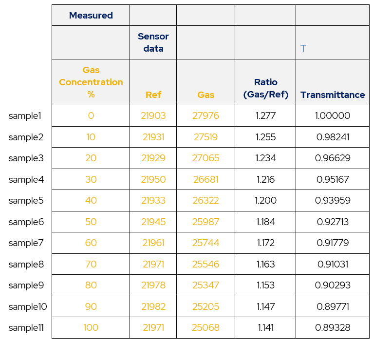
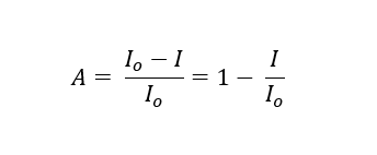
Table 1 – Calibration Data. Using the definition of transmittance
Where ‘I’ is the measured signal and ‘Io’ is the signal with 100% transmission (zero signal absorbed by the gas). Dividing the gas by the reference normalizes the output for the system being calibrated, with the value of gas/ref with 0% concentration of gas giving the value of ‘Io’ for the system since by definition there is 100% transmission when there is no gas present to absorb the IR.
Then the amount of IR absorbed is then the total amount of IR emitted (Io) minus the amount transmitted. This is normalized to a ratio by dividing both terms by Io.
This definition of absorption is taken from “Non-Dispersive Infrared Gas Measurement” by J. Y. Wong and R. L. Anderson. It is really the combination of signal losses from photon absorption and scattering.
Table 2 – Transmittance and Absorption
Plotting the absorption against the concentration from calibration gases gives the following graph.
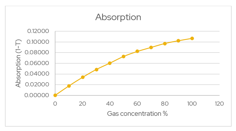
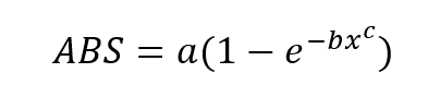
Figure 1 – Absorption vs. Concentration. The above graph is an exponential relationship however each system will be different so a few coefficients for calibration are required. The following equation for absorption is used.
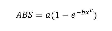
This is the format of the equation that the values of a, b and c will be determined from. This is due to the fact that the gas concentrations are the inputs for calibration process and the reduction in signal strength is the output of the calibration procedure.
In order to determine the coefficients, the add-in of excel ‘Solver’ must be enabled. This is done as shown below.
1. Click ‘Options’

2. Click ‘Add-Ins’

3. Click ‘Go…’ next to the manage Excel add-ins.

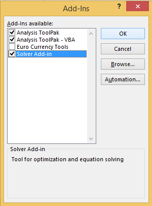
4. Ensure that the ‘Solver’ is selected in the Add-Ins available box. Then click ‘OK’.
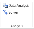
The solver options will now be available in the Analysis section of the top bar of Excel.
This is the tool that will be used to iterate towards values of the coefficients to provide a best fit curve. There are additional steps to set-up the spreadsheet so that the solver tool has what it needs to converge on an answer.
The solver tool needs to know the calculated values of absorbance and the actual values from calibration. Using these values as two columns create a third column that will be the square of the difference between the two columns.
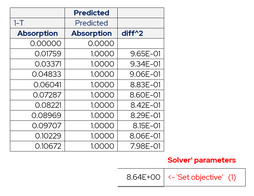
Table 3 – Layout of Actual Absorbance and Predicted Absorbance.
Finally add a final box that will contain the summation of the squares of the differences.
The final elements required are the boxes containing a, b and c.
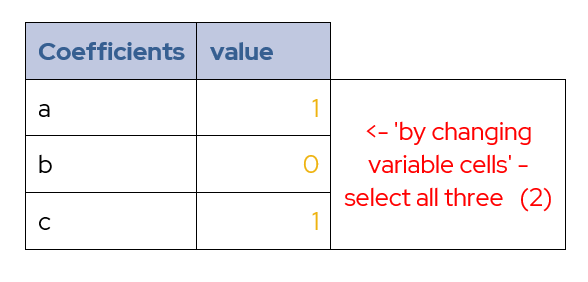
Table 4 – Cells for Coefficients
The predicted column shown in table x is then assigned the equation
with the concentration values coming from the calibration process, and the values for a, b and c coming from boxes created to contain them.
Starting the values for a and c at 1 and b set to zero, this will allow the solver to converge on an answer. These initial values are an example and may not be the best for every system. However, they work well the system used for this calibration procedure.
Click solver on the top bar of excel to open the solver options screen.
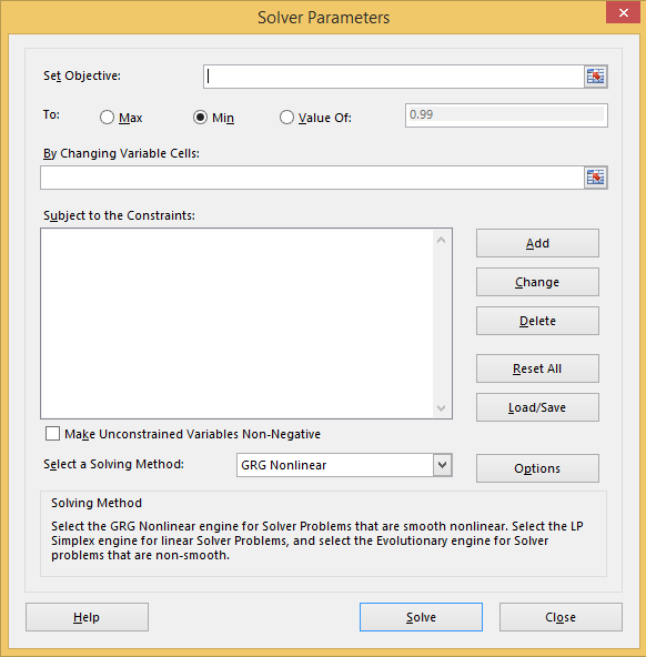
We want to minimize the summed error squared value. This is termed the ‘Objective’. Set the objective to the cell containing the squared error summation. And ensure that the selection of minimum is checked.
Next, we need to set the cells to be altered to help converge on a particular set of coefficients for the minimum error. This is the box with ‘By Changing Variable Cells’ above it. Select the three cells that contain the coefficients for this box.
Now click ‘Solve’. This will do one iteration of the algorithm. Repeat the above procedure until the values converge.
The values of coefficients determined from the above procedure are shown below.
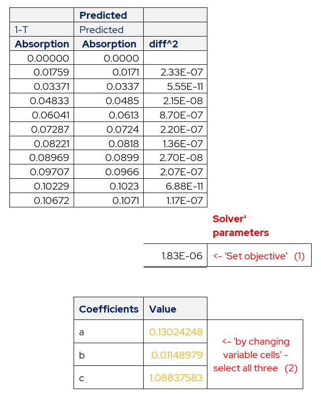
Table 5 – Determined Values of Coefficients
The above procedure has been based around the equation
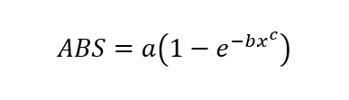
however, this is not an equation that outputs concentration values. Rearrange this equation to solve for ‘x’, which is the concentration.
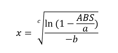
This is now the equation for determining the concentration of gas in the cell. With the values of a, b and c having been determined through the calibration process and using excel solver.
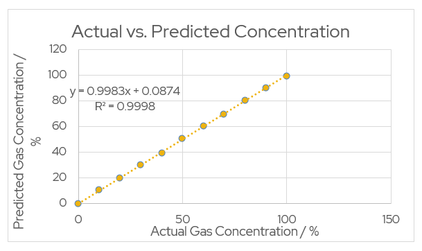
Figure 2 – Actual vs. Predicted Concentration
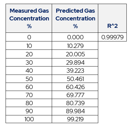
Table 6 – Table of Actual Concentration vs. Predicted.
This process produces an accurate equation for predicted values of gas concentration.